Interval Scheduling
The Greedy approach 贪心算法
-
The goal is to come up with a global solution. 提出一个全局的解法
-
The solution will be built up in small consecutive steps. 会构建连续小步
-
For each step, the solution will be the best possible
myopically(目光短浅地), according to some criterion (通过一些准则). -
Definition:
-
We start by selecting an interval [s(i), f(i)] for some request i.
-
We include this interval in the schedule.
-
This necessarily means that we can not include any other interval that is not compatible with [s(i), f(i)].
-
We will continue with some compatible interval [s(j), f(j)] and repeat the same process.
-
We terminate when there are no more compatible intervals to consider.
-
-
The Greedy Approach
-
Option 1: Choose the available interval that starts earliest.
-
Option 2: Choose the smallest available interval.
-
Option 3: Something more clever.
-
Interval Scheduling
-
A set of requests {1, 2, … , n}.
-
Each request has a starting time s(i) and a finishing time f(i).
-
Alternative view: Every request is an interval [s(i), f(i)].
-
-
Two requests i and j are compatible if their respective intervals do not overlap.
-
Goal: Output a schedule which maximises the number of compatible intervals.
Greedy Algorithm for interval scheduling
/**
IntervalScheduling([s(i), f(i)]i=1 to n)
  Let R be the set of requests, let A be empty
  While R is not empty
    Choose a request i with the smallest f(i).
    Add i to A
    Delete all requests from R that are not compatible with request i.
  Return the set A of accepted requests
*/
Arguing for optimality
-
Some notation:
-
O is the optimal schedule. Recall, that A is the schedule of the Greedy algorithm.
-
Let i1, i2, … , ik be the order in which the intervals were added to A by the algorithm.
-
Note that |A| = k.
-
Let j1, j2, … , jm be the set of requests in O.
-
Note that |O| = m.
-
We will prove that m=k. (Why is that enough?)
-
-
Let j1, j2, … , jm be the set of requests in O.
-
Assume wlog that this is in order of increasing s(jh).
-
Since O is feasible, this is also in order of increasing f(jh).
-
-
Claim: f(i1) ≤ f(j1)
- This holds because i1 is chosen to be the interval with the smallest f(ih).
-
Claim: f(i1) ≤ f(j1)
- As i1 is chosen to be the interval with the smallest f(ih).
-
Lemma: For all indices r ≤ k, it holds that f(ir) ≤ f(jr)
-
Proof by induction:
-
Base Case (r=1), by Claim.
-
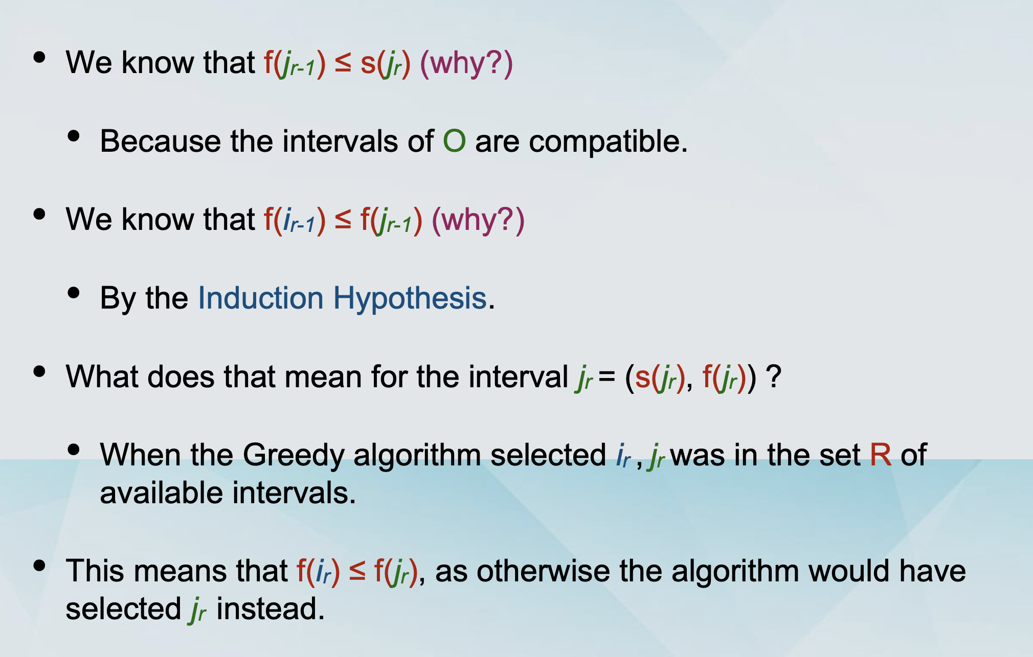
Induction Step. Assume it is true for r-1 i.e. (IH): f(ir-1) ≤ f(jr-1)
-
we will prove it for r.
-
-
Induction step proof
Completing the proof
-
By contradiction: To the contrary, assume that m > k
-
For r=k, the Lemma gives us that f(ik) ≤ f(jk).
-
Since m > k , there is an extra request jk+1 in O.
-
s(jk+1) > f(jk) ≥ f(ik).
-
The greedy algorithm would have continued with jk+1.
Running Time
The running time is O(n log n).
Minimum Spanning Tree 最小生成树
-
Consider a connected graph G=(V, E), such that for every edge e=(v,w) of E, there is an associated positive cost ce.
-
Goal: Find a subset T of E so that the graph G’=(V, T) is connected and the total cost
sum ceis minimised.
Claim: T is a tree
-
By definition, (V, T) is connected.
-
Suppose that it contained a cycle.
-
Let e be an edge on that cycle.
-
Take (V, T-{e}).
-
This is still connected.
- All paths that used e can be rerouted through the other direction.
-
(V, T-{e}) is a valid solution, and it is cheaper. Contradiction!
Greedy Approach 1 (Kruskal’s Algorithm)
-
Start with an empty set of edges T.
-
Add one edge to T.
-
Which one?
-
The one with the minimum cost
ce.
-
-
We continue like this.
-
Do we always add the new edge e to T?
- Only if we don’t introduce any cycles.
Greedy Approach 2 (Prim’s Algorithm)
-
Start with an empty set of edges T.
-
Start with a node s.
-
Add an edge e=(s,w) to T.
-
Which one?
-
The one with the minimum cost ce.
-
-
We continue like this – growing a set of connected vertices.
- We only consider edges to neighbours that are not in the spanning tree.
The cut property
Kruskal’s algorithm is optimal
-
Consider any edge e=(u, w) that Kruskal’s algorithm adds to the output on some step.
-
Let S be the set of nodes reachable from u just before e is added to the output.
-
It holds that u is in S and w is in V-S.(Why?)
- Because otherwise adding e would create a cycle.
-
The algorithm has not found any edge crossing S and V-S. (Why?)
- Such an edge would have been added to the output by the algorithm.
-
The edge e must be the cheapest edge crossing S and V-S.
-
By the cut property, it belongs to every minimum spanning tree.
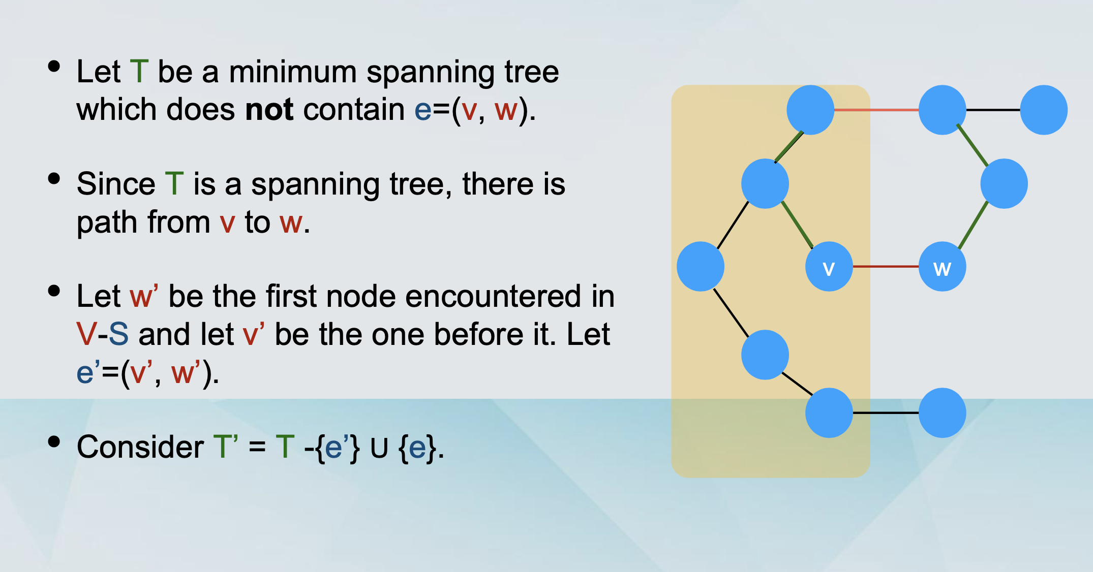
Prim’s algorithm is optimal
-
In each iteration of the algorithm, there is a set S of nodes which are the nodes of a partial spanning tree.
-
An edge is added to “expand” the partial spanning tree, which has the minimum cost.
-
This edge has one endpoint in S and one in V-S and has minimum cost.
-
So it must be part of every minimum spanning tree.
Greedy Approach 3 (Reverse-Delete Algorithm)
-
Start with the full graph G=(V, E).
-
Delete an edge from G.
-
Which one?
-
The one with the maximum cost ce.
-
-
We continue like this.
-
Do we always remove the considered edge e from G?
-
As long as we don’t disconnect the graph.
-
The cycle property
-
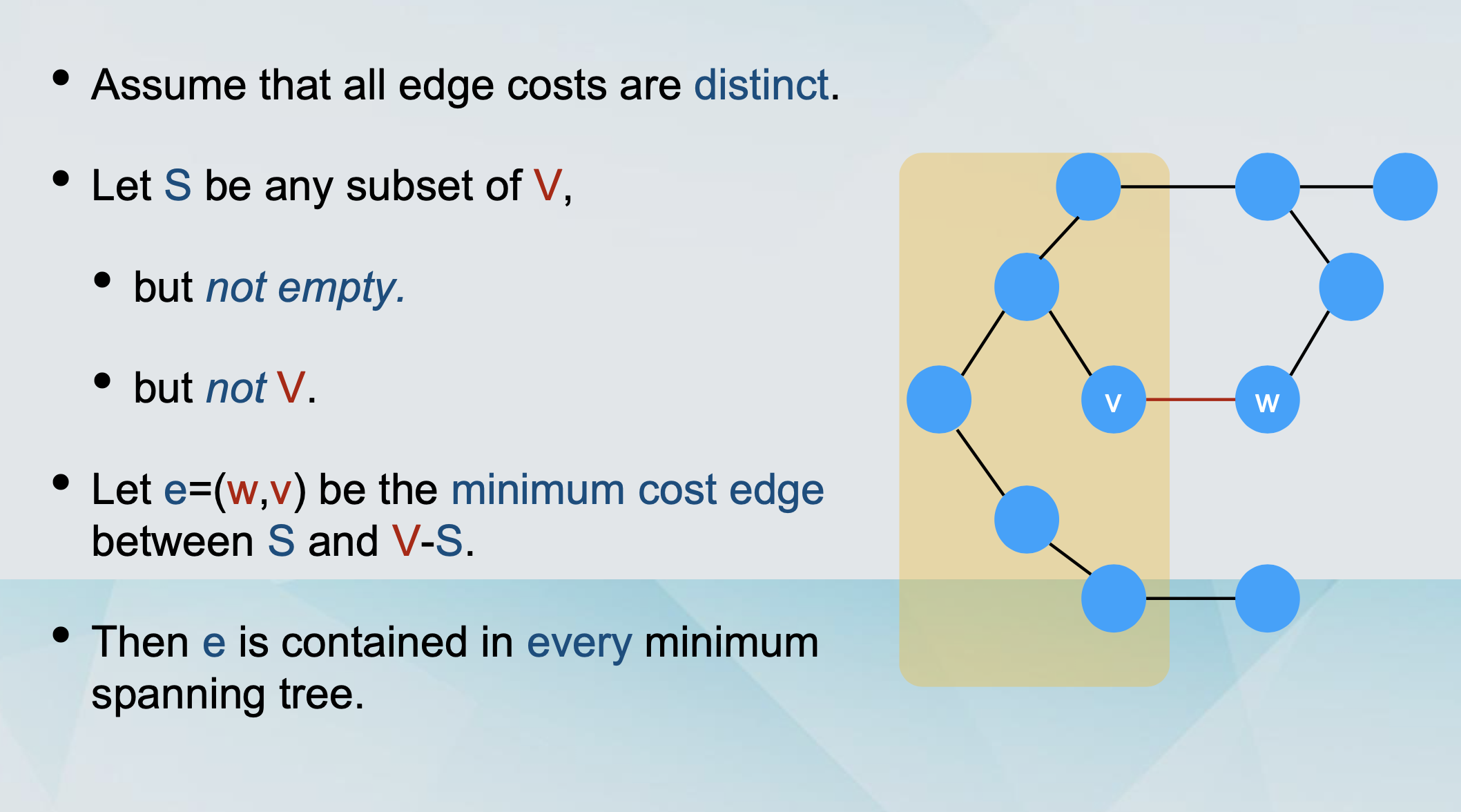
Assume that all edge costs are distinct.
-
Let C be any cycle of G.
-
Let e=(w,v) be the maximum cost edge of C.
-
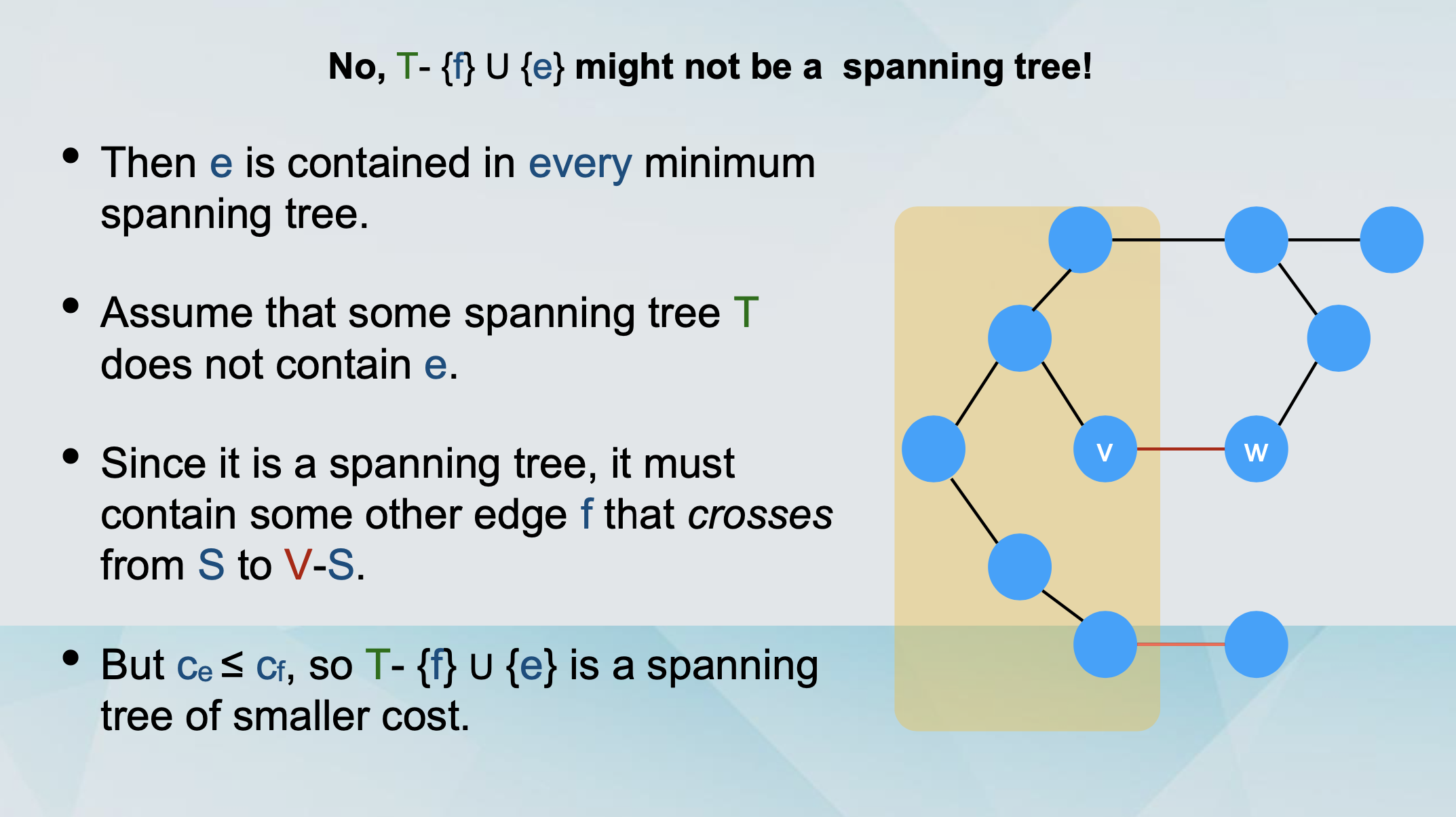
Then e is not contained in any minimum spanning tree of G.
-
Let T be a spanning tree that contains e.
-
We will show that it does not have minimum cost.
-
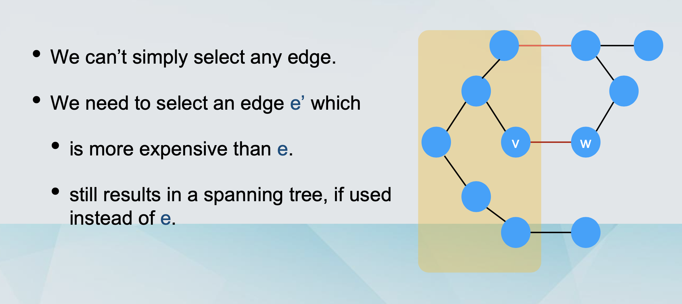
We will substitute e with another edge e’, resulting in a cheaper spanning tree.
-
How to find this edge e’?
-
We delete e from T.
-
This partitions the nodes into
-
S (containing u).
-
V - S (containing w).
-
-
We follow the other path the cycle from u to w.
-
At some point we cross from S to V - S, following edge e’.
-
The resulting graph is a tree with smaller cost.
Reverse-Delete is optimal
-
Consider any edge e=(v, w) which is removed by Reverse- Delete.
-
Just before deleting, it lies on some cycle C.
-
It has the maximum cost among edges, so it cannot be part of any minimum spanning tree.
Non-distinct costs
-
Take the original instance with non-distinct costs.
-
Make the costs distinct by adding small numbers ε to the costs to break ties.
-
Obtain a perturbed instance.
-
Run the algorithm on the perturbed instance.
-
Output the minimum spanning tree T.
-
T is a minimum spanning tree on the original instance.
T in the original instance
-
Suppose that there was a cheaper spanning tree
T*on the original instance. -
If
T*contains different edges to T but with the same costs, it is not cheaper than T on the original instance. -
If
Tcontains different edges with different costs, we can make ε small enough to make sure the ones we selected are still cheapest.
Prim’s algorithm running time
-
We add nodes to the expanding spanning tree S.
-
We need to figure out which node to add next.
-
We need to know the attachment cost of each node: a(v) = mine=(u,v):u is in S ce
-
Naive solution: For every step run over all candidates.
-
O(n2).
Priority Queue
-
Maintains
-
A set of elements S.
-
A key key(v) for each element v in S.
-
-
The key denotes the priority of v.
-
Operations:
-
Add(v) - with priority key. • Delete(v)
-
Extract_Min(v)
-
Change_key(v)
-
-
The Priority Queue is an abstract data type.
-
In reality, we have to implement it with known data structures.
-
Many implementations exists, the usual one is with heaps.
-
For now:
- PQ operations can be implemented in O(log n) time.
-
PQ solution: Insert the nodes in a PQ, with minus the attachment cost as the keys.
Clustering
Definition of Clustering
-
Definition: Given a set U of n elements, a k-clustering of U is a partition of U into non-empty sets C1, …, Ck.
-
Definition: The spacing of a k-clustering is the minimum distance between any pair of points in different clusters. // 不同集合之间的最小距离
-
Goal: Among all possible k-clusterings, find one with the maximum possible spacing.
In greedy algorithm
-
Pick two objects pi and pj with the smallest distance d(pi,pj).
-
Connect them with an edge e=(pi,pj).
-
Continue like this until we obtain k clusters.
-
If the edge e under consideration connects two objects pi and pj already in the same component, skip it.
Kruskal’s algorithm
-
Pick an edge (pi, pj) with the smallest cost d(pi,pj).
-
Include the edge in the output.
-
Stop before including the last k-1 edges.
- i.e., in the end, remove the k-1 most expensive edges.
-
If the edge e under consideration introduces a cycle, then skip it.
-
Lemma: Let C1, C2, … , Ck be the k connected components formed by deleting the k-1 most expensive edges from a minimum spanning tree T. // 生成一个最小生成树需要删除 k - 1 条最 expensive 的边
-
Proof of the Lemma
-
Let C’ = {C’1, C’2, … , C’k} be any other k-clustering.
-
By other, there exists a cluster Cr of C which is not contained in any cluster C’s of C’.
-
This means that there exist points pi, pj in Cr that belong to different clusters in C’.
-
Let C’i and C’j denote these clusters respectively.
-